Stream tweets in under 15 lines of code + some interactive data visualization

Introduction:

In this tutorial I will show you the easiest way to fetch tweets from twitter using twitter's API.
We will fetch some tweets, store them into a DataFrame and do some interactive visualization to get some insights.

In order to access twitter's API you need to have the below:

Consumer API key
Consumer API secret key
Access token
Access token secret

It is a very simple 5 minutes process getting those. You just need to log into your twitter account and go to this link click create an app and just follow the steps.
After you create an app and fill the app details, you can just go into your app details and go to the keys & tokens tab and click generate and you'll have your keys & tokens.

Getting the tweets:

We start by storing our keys & tokens into variables

access_token = 'paste your token here'
access_token_secret = 'paste your token secret here'
consumer_key = 'paste your consumer key here'
consumer_secret = 'paste your consumer secret here'

Next we import the libraries we'll use for now

import tweepy
import numpy as np
import pandas as pd

Tweepy is the library we'll use to access twitter's API.
If you don't have any of those libraries you can just run a pip install for the missing library.

Now we authenticate using our credentials as follows:

auth = tweepy.OAuthHandler(consumer_key, consumer_secret)
auth.set_access_token(access_token, access_token_secret)
api = tweepy.API(auth)

Once we are authenticated it's as simple as just picking any topic we want to search for on twitter to see what people are tweeting about in the context of that topic.

For example let's pick a very generic word "Food" and let's see what people are tweeting about in that context.

for tweet in api.search('food'):
    print(tweet.text)

api.search generally returns a lot of attributes for a tweet (one of them is the tweet itself). Other attributes are things like the user name of the tweeting user, how many followers they have, if the tweet was retweeted and many of other attributes (we will see how to get some of those later).
For now what I am interested in is just the tweet itself so I am returning "tweet.text".

The result is as follows:

By default "api.search" returns 15 tweets, but if we want more tweets we can get up to 100 tweets by adding count = 100. Count is just one of the arguments we can play around with among others like the language, location... etc. You can check them out here if you are interested in filtering the results according to your preference.

At this point we managed to fetch tweets under 15 lines of code.
If you want to get a larger number of tweets along with their attributes and do some data visualization keep reading.

Getting the tweets + some attributes:

In this section we will get some tweets plus some of their related attributes and store them in a structured format.

If we are interested in getting more than 100 tweets at a time which we are in our case, we will not be able to do so by just using "api.search". We will need to use "tweepy.Cursor" which will allow us to get as many tweets as we desire. I did not get too deep into trying to understand what Cursoring does, but the general idea in our case is that it will allow us to read 100 tweets store them in a page inherently then read the next 100 tweets.
For our purpose the end result is that it will just keep going on fetching tweets until we ask it to stop by breaking the loop.

I will first start by creating an empty DataFrame with the columns we'll need.

df = pd.DataFrame(columns = ['Tweets', 'User', 'User_statuses_count', 
                             'user_followers', 'User_location', 'User_verified',
                             'fav_count', 'rt_count', 'tweet_date'])

Next I will define a function as follows.

def stream(data, file_name):
    i = 0
    for tweet in tweepy.Cursor(api.search, q=data, count=100, lang='en').items():
        print(i, end='\r')
        df.loc[i, 'Tweets'] = tweet.text
        df.loc[i, 'User'] = tweet.user.name
        df.loc[i, 'User_statuses_count'] = tweet.user.statuses_count
        df.loc[i, 'user_followers'] = tweet.user.followers_count
        df.loc[i, 'User_location'] = tweet.user.location
        df.loc[i, 'User_verified'] = tweet.user.verified
        df.loc[i, 'fav_count'] = tweet.favorite_count
        df.loc[i, 'rt_count'] = tweet.retweet_count
        df.loc[i, 'tweet_date'] = tweet.created_at
        df.to_excel('{}.xlsx'.format(file_name))
        i+=1
        if i == 1000:
            break
        else:
            pass

Let's look at this function from the inside out:

First we followed the same methodology of getting each tweet in a for loop, but this time from "tweepy.Cursor".
Inside "tweepy.Cursor" we pass our "api.search" and the attributes we want:

q = data: data will be whatever piece of text we pass into the stream function to ask our api.search to search for just like we did passing "food" in the previous example.
count = 100: Here we are setting the number of tweets to return per api.search to 100 which is the maximum possible number.
lang = 'en': Here I am simply filtering results to return tweets in English only.

Now since we put our api.search into tweepy.Cursor it will not just stop at the first 100 tweets. It will instead keep going on forever that's why we are using "i" as a counter to stop the loop after 1000 iterations.
Next I am filling my dataframe with the attributes I am interested in during each iteration making use of .loc method of pandas and my "i" counter.
The attributes I am passing into each column are self explanatory and you can look into the twitter api documentation for what other attributes are available and play around with those.
Finally I am saving the result into an excel file using "df.to_excel" and here I am using a placeholder {} instead of naming the file inside the function because I want to be able to name the file myself when I run the function.

Now I can just call my function as follows looking for tweets about food again and naming my file "my_tweets" as follows:

stream(data = ['food'], file_name = 'my_tweets')

It will keep running until 1000 tweets are returned (of course you can set the limit to whatever number of tweets you may want to get).

Ok now I can open the excel sheet in my directory to see the result or peak at the result in my dataframe as follows:

df.head()

Ok great everything is working as planned.

Let's analyze some tweets:

In this section we will do some interactive visualization on 200k+ tweets that I already had streamed & saved to get some insights.

I will be using plotly based on this article to produce some visualizations without going into the details of using plotly, but if you are interested in more details about the capabilities of plotly you can check the article it is a great resource.

Let's import our libraries:

from textblob import TextBlob
from wordcloud import WordCloud, STOPWORDS
import plotly.plotly as py
import plotly.graph_objs as go
from plotly.offline import iplot
import cufflinks
cufflinks.go_offline()
cufflinks.set_config_file(world_readable=True, theme='pearl', offline=True)

Let's look at our dataframe:

df.info()

Ok here we have 226,782 tweets and some values missing for "User" & "User_location.
It makes sense to have some user locations missing since not all twitter users put their location on their profile.
For User I am not sure why those 17 entries are missing, but anyway for our scope here we will not need to deal with missing values.

Let's also take a quick peak at the first 5 rows of our dataframe:

df.head()

I would like to add an extra column to this dataframe that indicates the sentiment of a tweet.
We will also need to add another column with the tweets stripped off of useless symbols then run the sentiment analyzer on those cleaned up tweets to be more effective.

Let's start by writing our tweets cleaning function:

def clean_tweet(tweet):
    return ' '.join(re.sub('(@[A-Za-z0-9]+)|([^0-9A-Za-z \t])|(\w+:\/\/\S+)', ' ', tweet).split())

Let's also write our sentiment analyzer function:

def analyze_sentiment(tweet):
    analysis = TextBlob(tweet)
    if analysis.sentiment.polarity > 0:
        return 'Positive'
    elif analysis.sentiment.polarity ==0:
        return 'Neutral'
    else:
        return 'Negative'

Now let's create our new columns:

df['clean_tweet'] = df['Tweets'].apply(lambda x: clean_tweet(x))
df['Sentiment'] = df['clean_tweet'].apply(lambda x: analyze_sentiment(x))

Let's look at some random rows to make sure our functions worked correctly
Example (3,000th row):

n=3000
print('Original tweet:\n'+ df['Tweets'][n])
print()
print('Clean tweet:\n'+df['clean_tweet'][n])
print()
print('Sentiment:\n'+df['Sentiment'][n])

Example (20th row):

n=20
print('Original tweet:\n'+ df['Tweets'][n])
print()
print('Clean tweet:\n'+df['clean_tweet'][n])
print()
print('Sentiment:\n'+df['Sentiment'][n])

Ok it seems like our functions are working. (Note that doing sentiment analysis by directly feeding our text to textblob sentiment analyzer like that will not yield 100% perfect results for all tweets. In order to do so we need to do some more detailed text pre-processing, but anyway for the purpose of this tutorial what we have so far will suffice).

At this point we are ready to do some data visualization.

A few things I am interested to see are:

The Sentiment distribution of all the tweets (do most tweets have a positive, negative or neutral context?)
The Sentiment distribution of most popular tweets.
The Sentiment distribution of tweets with average popularity.
The Sentiment distribution of least popular tweets.
Is there a correlation between the a user's tweeting frequency & having a high number of followers?
Does the user being a verified user or not have an impact on the above correlation?
What are the most frequent words used by all twitter users?
What are the most frequent words used by popular twitter users?
What are the most frequent words used by twitter users of average popularity?
What are the most frequent words used by least popular twitter users?

Sentiment distribution

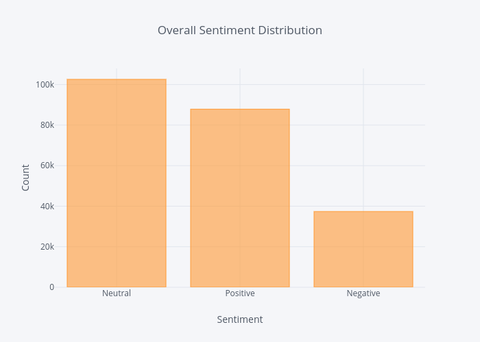
Overall:

df['Sentiment'].value_counts().iplot(kind='bar', xTitle='Sentiment',
                                    yTitle='Count', title='Overall Sentiment Distribution')

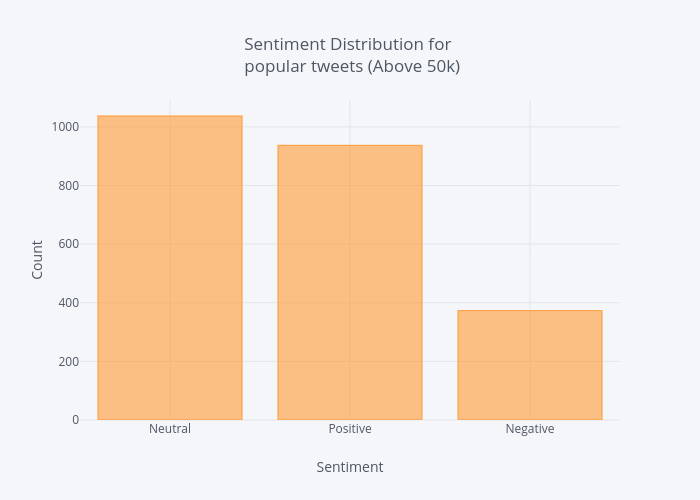
Most popular:

Below I just create a new dataframe from our original one filtering with retweet counts above or equal to 50k.

df_popular = df[df['rt_count'] >= 50000]
df_popular['Sentiment'].value_counts().iplot(kind='bar', xTitle='Sentiment',
                                    yTitle='Count', title = 'Sentiment Distribution for <br> popular tweets (Above 50k)')

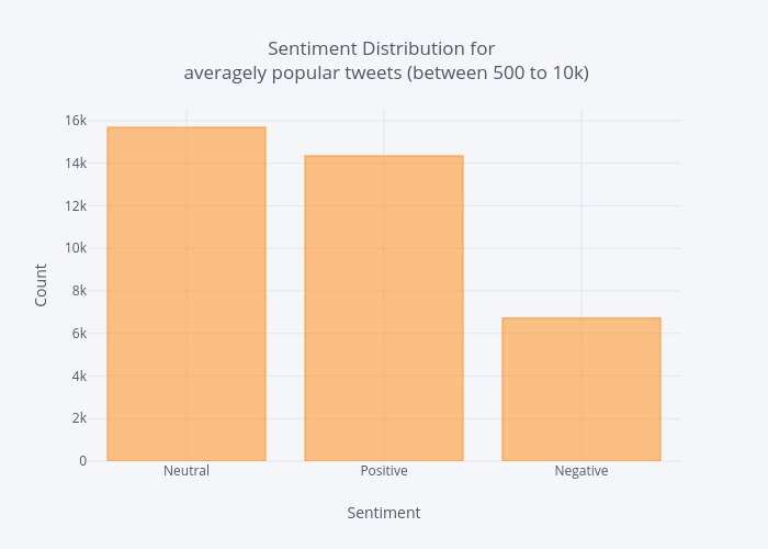
Average popularity:

Create a new dataframe from our original one filtering with retweet counts between 500 and 10k.

df_average = df[(df['rt_count'] <= 10000) & (df['rt_count'] >=500)]
df_average['Sentiment'].value_counts().iplot(kind='bar', xTitle='Sentiment',
                                    yTitle='Count', title = ('Sentiment Distribution for <br> averagely popular tweets (between 500 to 10k)'))

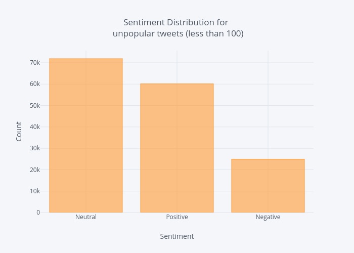
Least popular:

Create a new dataframe from our original one filtering with retweet counts less than or equal to 100.

df_unpopular = df[df['rt_count'] <= 100]
df_unpopular['Sentiment'].value_counts().iplot(kind='bar', xTitle='Sentiment',
                                    yTitle='Count', title = ('Sentiment Distribution for <br> unpopular tweets (between 500 to 10k)'))

From the above charts we can conclude that:

Generally speaking most tweets are neutral.
Most people tend to tweet about positive things rather than negative.
Tweet sentiment has little impact on retweet count.

Correlation between tweeting frequency & followers:

Let's:

Plot the number of statuses per user vs. number of followers per user.
Differentiate between verified & non verified users in our plot.

df.iplot(x='User_statuses_count', y = 'user_followers', mode='markers'
        , categories='User_verified',layout=dict(
        xaxis=dict(type='log', title='No. of Statuses'),
        yaxis=dict(type='log', title='No. of followers'),
        title='No. of statuses vs. No. of followers'))

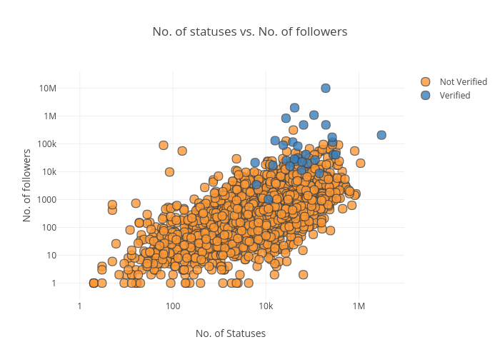
Here I am putting the values on a log scale to reduce the impact of outliers.

Note: in the above chart I am not using the full 200k+ data set as it gets really slow to load it as an interactive chart. Instead I just sampled only 3k entries.

From the above chart we conclude 2 things:

The frequency of tweeting could indeed be one of the contributing factors in the number of followers.
Verified users tend to follow the same distribution as non verified users, but they are mostly concentrated in the upper region with a higher number of followers above non verified users (which makes sense as most verified users are expected to be public figures).

Let's check most frequently used words:

To visualize the most frequently used words we will use wordcloud which is a great way to do such task. Word Cloud gives us an image showing all words used in a piece of text in different sizes where words shown in bigger sizes are used more frequently.

In order to get meaningful results we need to filter our tweets by removing stopwords. Stop words are generally commonly used words that act as fillers in a sentence and it is common practice to remove such words in natural language processing as although we use them for our understanding of a sentence as human beings they do not add any meaning for computers when processing language and they actually act as noise in the data.

The word cloud library has a built in stop words list that we already imported above which can be used to filter out stop words in our text.

First we need to create join all our tweets as follows:

all_tweets = ' '.join(tweet for tweet in df['clean_tweet'])

Next we create the word cloud:

wordcloud = WordCloud(stopwords=stopwords).generate(all_tweets)

Note that above I am not using the built in list of stopwords included with the wordcloud library. I am using a much larger list that includes tons of stop words in several languages, but I am not going to paste it here to avoid taking useless space in this tutorial as it is a very big list (you can find such lists if you search online). Anyway if you want to use the built in list you can just ignore the above code and use the below:

wordcloud = WordCloud(stopwords=STOPWORDS).generate(all_tweets)

Finally we plot the wordcloud & show it as an image:

plt.figure(figsize = (10,10))
plt.imshow(wordcloud, interpolation='bilinear')
plt.axis("off")
plt.show()

We can also plot the frequencies of words as follows:

df_freq = pd.DataFrame.from_dict(data = wordcloud.words_, orient='index')
df_freq = df_freq.head(20)
df_freq.plot.bar()

Let's do the same thing again only for popular tweets by just changing this piece of code:

all_tweets = ' '.join(tweet for tweet in df_popular['clean_tweet'])

WordCloud:

Word Frequencies:

Now you get the idea how to do this also for average & unpopular tweets.

That's all!.

I hope you found this tutorial useful.

Omar Aref

Search This Blog